Preference SQL Syntax

This page provides a short overview of base and complex preference constructors with their syntax. For all of them a substitutable values relation (SV-Relation) can be specified.

Preference SQL = SQL + Preferences

Preference SQL extends the SQL92 standard by means to express preferences in the form of soft constraints. For this purpose, the SQL query block is extended with a PREFERRING, GROUPING, BUT ONLY, and TOP clause.

Preference SQL Query Block

A Preference SQL query block has the following schematic design:

	 	 	 	 	 Step: 
SELECT 	 	 <projection_list> 	 (11) 
FROM 	 	 <table_references> 	 (01) 
WHERE 	 	 <hard_conditions> 	 (02) 
PREFERRING 	 <soft_conditions> 	 (04) 
GROUPING 	 <attribute_list> 	 (03) 
TOP 	 	 <number> 	 	 (05) 
BUT ONLY 	 <but_only_conditions> 	 (06) 
GROUP BY 	 <attribute_list> 	 (07) 
HAVING 	 	 <hard_conditions> 	 (08) 
ORDER BY 	 <attribute_list> 	 (09) 
LIMIT 	 	 <number> 	 	 (10)

While PREFERRING, GROUPING, BUT ONLY and TOP describe specific syntax for preference handling, other clauses such as GROUP BY or LIMIT behave according to the SQL92 standard. For details about specific clauses we refer to the Preference SQL Overview . The next paragraph describes the interplay between soft and hard constraints and their evaluation order.

Preference SQL Evaluation Order

The number in the column Step indicates the order of evaluation. Hence, a (full) Preference SQL query is evaluated in the following order:

Tuples are read from the relations specified in the FROM clause.
Tuples are filtered according to the hard constraints of the WHERE clause.
Tuples are separated into groups depending on the attributes specified in the GROUPING clause.
The best tuples with regard to the preference specified in the PREFERRING clause are selected per group. Groups then are joined into a single set of tuples.
The TOP clause specifies a fixed number K of tuples to be retrieved. If there are more than K tuples in the result set, the result set is limited to K tuples. If there are less than K tuples in the result set, more next best items are inserted into the result set.
Tuples that do not satisfy the hard condition specified in the BUT ONLY clause are removed.
Tuples are grouped according to the GROUP BY clause.
Groups not satisfying the HAVING clause are discarded.
Tuples are sorted according to the values of the attributes given in the ORDER BY clause.
If there a more tuples than the number specified in the LIMIT clause, the result set is truncated.
Tuples are projected to the attributes, aggregation results, and function values specified in the SELECT clause.

For a valid Preference SQL query, only SELECT, FROM, and PREFERRING are necessary, all other clauses are optional and their evaluation steps can be omitted. Of course Preference SQL can also handle plain SQL92 queries without preferences specified.

SV-Relation

A SV-Relation can be TRIVIAL, REGULAR or explicit. For more information cp. SV-Relation.

<SV-Relation> ::= 
∅ | default, REGULAR SV-Relation
REGULAR | indifference
TRIVIAL | trivial SV-Relation, identity
SV ((<string_literal>, <string_literal>) [, ( <string_literal>, <string_literal> ) ]* ) | explicit SV-Relation

SELECT Id 
FROM car 
PREFERRING color IN ('blue', 'yellow' , 'white') ELSE ('green', 'red' , 'pink') ('blue', 'yellow' , 'white') ELSE ('green', 'red' , 'pink') SV ( ('blue', 'yellow') ('green', 'red' , 'pink') SV ( ('blue', 'yellow'), ('green', 'red') ) AND price LOWEST;

NULL-handling

Preference SQL supports five different types of NULL-handling statements for numerical and categorical base preferences:

AVOID NULL: Makes NULL values least preferred, i.e. every other attribute values is rated better than a NULL value.
WITH NULL WORST: Places NULL values among the worst available attribute values.
WITH NULL AT BMO: Makes NULL values as good as the best available attribute values, i.e. NULL values always occur in the preference's BMO-set
WITH NULL AT DISTANCE v: Places NULL values at the distance v to the base preference's optimal values. This statement is only applicable to numerical base preferences.
WITH NULL AT LEVEL v: Places NULL values at the level v. Note that the usage of this statement requires regular SV-semantics for the base preference and in case of a numerical preference a d-parameter greater 0.

If the NULL-handling term is omitted for a base preference, WITH NULL WORST is used by default. If NULL is place in one of the layers for a categorical preference and a NULL-handling term is specified, too, placing a NULL value in a layer always takes precedence over any potentially given NULL-handling statement.

For more detailed explanations regarding the NULL-handling in Preference SQL, see Handling NULL values in Preference SQL.

<NULL-handling> ::= AVOID NULL 
| WITH NULL WORST 
| WITH NULL AT BMO 
| WITH NULL AT DISTANCE <number> 
| WITH NULL AT LEVEL <number>

SELECT * 
FROM car 
PREFERRING color LAYERED ( ('black', 'white') , ('blue', 'silver') , OTHERS, ('green', 'red', 'yellow', 'orange') ) WITH NULL AT LEVEL 1;

SELECT * FROM car PREFERRING age BETWEEN 1 AND 4 WITH NULL AT DISTANCE 5;

Base Preference Constructors

The preferring clause is inductivly constructed by base preference constructors which themselves are combined by complex preference constructors. To visualize preference orders of base preferences, this reference guide uses Hasse diagrams.

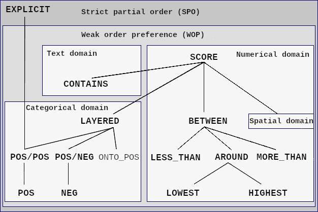
Base preference constructors are the building blocks to express preferences. Depending on the underlying domain, base preferences are either defined on numerical, categorical, textual, spatial, or temporal domains. The following taxonomy provides an overview of existing base preference constructors.

Strict Partial Orders

SPOs have two important properties:

Irreflexivity
Transitivity

This reference guide uses Hasse diagrams to describe SPOs and to specify the relation between items:

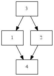
In the picture above, item 3 is preferred to both 1 and 2 which in turn are both preferred to item 4, while of course (by transitivity), item 3 is also preferred to item 4. Hence, the diagrams contain arrows from more preferred items to less preferred items. Furthermore, as we know that transitivity holds for strict partial orders, to reduce cluttering, the diagrams do not contain arrows for which a transitive alternative exists.

We extend this syntax by also allowing set valued labels for the nodes in Hasse diagrams:

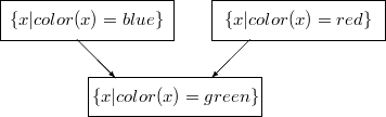
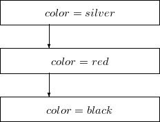
Instead of {x|attr(x) = ...}, we usually write attr = ... :

Weak Order Preference

WOPs have two important properties:

Strict Partial Order
Each WOP is a strict partial order.
Transitivity

REGULAR SV semantics is inherently obtained by a WOP by assigning an equivalence class for each layer denoted by the implicit level of the layer. WOP preferences are shown in the preference taxonomy.

Numerical base preferences

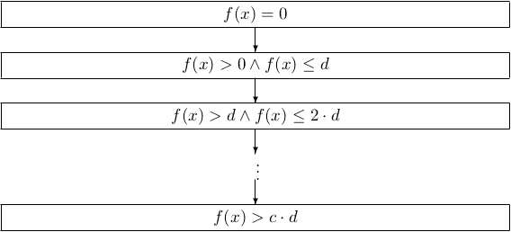
SCORE

(A, f, d, c, SV, N)

We assume a scoring function Let ‘<’ be the familiar ‘less-than’ order on ℝ. P is called SCORE preference, if for iff The lower the scoring value, the more an attribute value is preferred by the user.

Hasse diagram

Syntax

PREFERRING 
<column> SCORE <string_literal> [<d>] [, <c>] [<SV-Relation>] [<NULL-handling>]

Note that the score function (<string_literal>), have to be implemented by the user, either within the Preference SQL code itself, or by the create scorefunction-command. For a list of predefined score- and rank-functions see predefined SCORE and RANK functions.

Examples

Regarding a CD collection with attribute feedback, I prefer CDs having a better feedback. The CD c1 is better than CD c2 if c1's score is less than c2's score.

PREFERRING feedback SCORE 'feedback_function'

SELECT * FROM car PREFERRING age SCORE 'age_function' 0.1

SELECT * FROM car PREFERRING price SCORE 'price_function' 5 REGULAR

BETWEEN

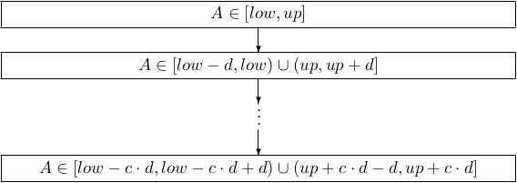
(A, [low, up, d, c, SV, N)]

A desired value should be between the bounds of an interval. If this is infeasible, values with shortest distance apart from the interval boundaries will be acceptable.

Hasse diagram

Regarding any attribute A, users may prefer values between a lower limit (LOW) and an upper limit (UP). Other values are scored by their distance to UP or LOW.

Syntax

PREFERRING 
<column> BETWEEN <low> AND <up> [, <d> ] [, <c> ] [ <SV-Relation>] [<NULL-handling>]

Examples

My favorite walking distance is about 15 - 20 km.

PREFERRING walking_distance BETWEEN 15 AND 20

SELECT * FROM car PREFERRING age BETWEEN 10 AND 16

SELECT * FROM car PREFERRING price BETWEEN 5000 AND 6000 , 100 TRIVIAL

LESS THAN and MORE THAN

(A, z, d, c, SV, N)

A desired value should be less than or more than a given value z. If this is infeasible, values with shortest distance apart from z will be acceptable.

Syntax

PREFERRING 
<column> LESS THAN <z> [, <d> ] [, <c> ] [<SV-Relation>] [<NULL-handling>] 
<column> MORE THAN <z> [, <d> ] [, <c> ] [<SV-Relation>] [<NULL-handling>]

Examples

My favorite earnings are more than 100.000 €.

PREFERRING earnings MORE THAN 100000

My preferred tax rate is less than 20 percent.

PREFERRING tax_rate LESS THAN 20

SELECT * FROM car PREFERRING age LESS THAN 10

SELECT * FROM car PREFERRING price MORE THAN 5, 1, 3 REGULAR

AROUND

(A, z, d, c, SV, N)

The desired value should be z. If this is infeasible, values with shortest distance apart from z are acceptable. AROUND can be expressed as BETWEEN with z as lower and upper bound.

Syntax

PREFERRING 
<column> AROUND <z> [, <d> ] [, <c> ] [<SV-Relation>] [<NULL-handling>]

Examples

For my new appartment, my favorite size is about 80 m2.

PREFERRING size AROUND 80

SELECT * FROM car PREFERRING age AROUND 9

SELECT * FROM car PREFERRING price AROUND 6500 , 500 REGULAR

HIGHEST

(A, d, c, SV, N)

A desired value should be as high as possible. The value z of the AROUND preference is set to z := max(A). Other values are accordingly scored by their distance to the highest value.

Syntax

PREFERRING 
<column> HIGHEST [<supremum> , <d>] [, <c>] [<SV-Relation>] [<NULL-handling>]

Examples

For my new car, the horse power should be as high as possible.

PREFERRING horse_power HIGHEST

SELECT * FROM car PREFERRING price HIGHEST

SELECT * FROM car PREFERRING horsepower HIGHEST 100, 10 REGULAR

LOWEST

(A, d, c, SV, N)

A desired value should be as low as possible. The value z of the AROUND preference is set to z := min(A). Other values are accordingly scored by their distance to the lowest value.

Syntax

PREFERRING 
<column> LOWEST [<infimum> , <d> ] [, <c>] [<SV-Relation>] [<NULL-handling>]

Examples

For my new car, the consumption should be as low as possible.

PREFERRING consumption LOWEST

SELECT * FROM car PREFERRING price LOWEST

SELECT * FROM car PREFERRING horsepower LOWEST 100, 10 REGULAR

Categorical base preferences

Categorical preference constructors are based on a discrete domain. This may be the case when the domain consists of categorical terms. Also any function may be discretized, especially the SCORE preference constructor by the d-parameter . Discrete domains lead to discrete levels l(x) that are used for preference evaluation rather than continuous scoring values f(x). Accordingly, attribute values x with lower level are more preferable. Each categorical preference constructor is a specialization of SCORE_d. Preference SQL supports these data types. We start with the description of the categorical preference constructors again in a top-down manner.

LAYERED

(A, L, SV, N)

LAYERED is a sub-constructor of SCORE. The LAYERED_m preference constructor is the most general categorical base preference constructor. It allows to specify an ordered list L = (L₁, · · · , L_m+1) (m = 0) of distinct subsets of the domain values of a categorical attribute. For convenience, one of the L_i may be named “OTHERS”, representing the elements of the attribute domain which are not part of any other subset.The preference order is then determined by

Syntax

PREFERRING 
<column> LAYERED ( 
(<string_literal> | <number> | NULL [, <string_literal> | <number> | NULL]*) 
| OTHERS | (OTHERS, NULL) | (NULL, OTHERS) 
[, (<string_literal> | <number> | NULL [, <string_literal> | <number> | NULL]*) 
| , OTHERS | , (OTHERS, NULL) | , (NULL, OTHERS)]*) 
[<SV-Relation>][<NULL-handling>]

Examples

My most favorite colors are blue and green, but I absolutely dislike red. Instead of getting any other color, I accept yellow. There are still other colors left in the attribute domain. Thus, the user explicitly describes three layers and arranges the implicit OTHER set second to last.

PREFERRING color IN ( ('blue', 'green') , ('yellow') , ('red') , OTHERS)

SELECT * 
FROM car 
PREFERRING color LAYERED ( ('red', 'black') , OTHERS, ('green', 'blue') )

POS

(A, POS-set, SV, N)

A POS preference expresses a soft condition that a desired value should be one out of a given list of values. Accordingly, it can be expressed as a LAYERED1 preference with L1 := POS-set and L2 := OTHERS.

Syntax

PREFERRING 
<column> = <string_literal> | <number> 
<column> IS NULL 
<column> IN (<string_literal> | <number> | NULL [, <string_literal> | <number> | NULL]* ) [<SV-Relation>] [<NULL-handling>]

Examples

My favorite colors are blue and green.

PREFERRING color IN ('blue', 'green')

SELECT * FROM car PREFERRING color IN ('yellow', 'green', 'blue')

SELECT * FROM car PREFERRING make = 'vw' REGULAR

NEG

(A, NEG-set, SV, N)

The NEG constructor lets users specify a NEG-set of disliked attribute values. Accordingly, it can be expressed as a LAYERED1 preference with L1 := OTHERS and L2 := NEG-set.

Syntax

PREFERRING 
<column> != <string_literal> | <number> 
<column> <> <string_literal> | <number> 
<column> IS NOT NULL

PREFERRING 
<column> NOT IN (<string_literal> | <number> | NULL [, <string_literal> | <number> | NULL]* ) [<SV-Relation>] [<NULL-handling>]

Examples

I dislike red and purple as color.

PREFERRING color NOT IN ('red', 'purple')

SELECT * FROM car PREFERRING color NOT IN ('yellow', 'green', 'blue')

SELECT * FROM car PREFERRING make <> 'vw' REGULAR

POS/POS

(A, POS1-set, POS2-set, SV, N)

A desired value should be amongst a finite set POS1-set. Otherwise values in the POS2-set are preferred over any value from the OTHERS set. Accordingly, the preference can be expressed as a LAYERED2 preference with L1 := POS1-set, L2 := POS2-set and L3 := OTHERS.

Syntax

PREFERRING 
<column> IN (<string_literal> | <number> | NULL [, <string_literal> | <number> | NULL]* ) 
ELSE (<string_literal> | <number> | NULL [, <string_literal> | <number> | NULL]* ) [<SV-Relation>] [<NULL-handling>]

Examples

My favorite colors are blue and green. Instead of getting any other color I prefer the color yellow.

PREFERRING color IN ('blue', 'green') ELSE ('yellow')

SELECT * FROM car PREFERRING make IN ('vw', 'audi') ELSE ('bmw', 'opel')

SELECT * 
FROM car 
PREFERRING color IN ('blue', 'yellow') ELSE ('red', 'green') REGULAR

POS/NEG

(A, POS-set, NEG-set, SV, N)

The POS/NEG constructor lets users specify a POS-set of preferred attribute values and a NEG-set of disliked values. Accordingly, it can be expressed as a LAYERED2 preference with L1 := POS-set, L2 := OTHERS, and L3 := NEG-set.

Syntax

PREFERRING 
<column> IN (<string_literal> | <number> | NULL [, <string_literal> | <number> | NULL]* ) 
NOT IN (<string_literal> | <number> | NULL [, <string_literal> | <number> | NULL]* ) [<SV-Relation>] [<NULL-handling>]

Examples

My favorite colors are blue and green but I dislike red.

PREFERRING color IN ('blue', 'green') NOT IN ('red')

SELECT * FROM car PREFERRING make IN ('vw', 'audi') NOT IN ('bmw', 'opel')

SELECT * 
FROM car 
PREFERRING color IN ('blue', 'yellow') ELSE ('red', 'green') REGULAR

EXPLICIT

(A, E-graph)

Regarding any attribute A, the most generic description of a user's preference is defined by a pairwise enumeration of values (v₁, v₂). The pair (v₁, v₂) defines that v₂ is preferred to v₁. This relation is visualized by the edges of an E-graph.

Note that all values in the range of the graph (i.e. explicitly specified in the preference) are considered to be better than all values not in the range of the graph (Other values). The EXPLICIT preference constructor has to constitute a strict partial order , otherwise an error (Cyclic graphs are not allowed.) is thrown. Only TRIVIAL SV semantics is supported by EXPLICIT.

The implementation ensures cycle-free e-graph.

Syntax

PREFERRING 
<column> EXPLICIT ( <string_literal> | <number> | NULL < <string_literal> | <number> | NULL [, <string_literal> | <number> | NULL < <string_literal> | <number> | NULL ]* )

Examples

I prefer blue to yellow and green to yellow. I also prefer yellow to red. I may also express that I prefer blue to red which is a redundant utterance, but I should never declare that I prefer red to blue to sustain consistency. All unspecified colors are incomparable aka indifferent.

This preference implies for example that blue is better than red (by transitivity) and that red is better than black (because black is unspecified in the preference and therefore considered to be worse).

PREFERRING color EXPLICIT ('red' < 'yellow', 'yellow' < 'blue')

SELECT * 
FROM car 
PREFERRING make EXPLICIT ( 'opel' < 'audi', 'audi' < 'bmw', 'audi' < 'bmw', 'audi' < 'vw', 'bmw' < 'vw')

ANTICHAIN

(A, SV)

Regarding any attribute A, it is possible that users state that they do not have any preference with regard to A. Thus, the ANTICHAIN preference expresses this empty preference which means that all values are incomparable aka indifferent and no effects are observable by this preference.

If ANTICHAIN however is prioritized to any preference this preference unveils the property of GROUPING by constituting equivalence classes by any SV semantics whereas the GROUPING clause only expresses TRIVIAL SV semantics as GROUP BY.

Hasse diagram

Syntax

PREFERRING <column> ANTICHAIN [<SV-Relation>]

Examples

I have no preference with respect to color.

PREFERRING color ANTICHAIN

PREFERRING age ANTICHAIN

ONTOPOS

Regarding a categorical attribute A, a generic ontologyor a more specific taxonomyexists which breaks down the terms of its domain into three relations of topics, subtopics, and synonyms. A term and its synonyms constitute LAYER₁. All immediate topics (parents) are members of LAYER₂ aka topics. All children of immediate topics but the considered term (first cousins) form LAYER₄ aka related terms. LAYER₃ consists of all descendants of the interesting term aka subtopics. LAYER₅ contains all other terms.

The interesting term may exist several times in the taxonomy introducing the problem of disambiguation. Preference SQL adapts to OWL as most accepted family of knowledge representation languages for authoring ontologies as well as to the domain-specific taxonomies of MPEG-7 defining the feasible keywords from a controlled vocabulary.

The ONTOPOS preference constructor is still under construction.

Textual base preferences

Text preference constructors are defined on character chains. The most important application is full text search.

CONTAINS

The CONTAINS preference allows a full-text search on text attributes based on the Apache Luceneframework. For this purpose, a Lucene index has to be defined via Preference SQL as base for preference evaluation. Only one Default-Index can be specified for a certain text attribute for implicit searching. Additionally, more than one index can exist on a textual attribute. Which index should be used has to be specified in a Preference SQL query by explicitly naming the name of the index through USING INDEX. Else the Default-Index is used.

Index

Before using CONTAINS an index has to be created.

CREATE CONTAINSINDEX [IF NOT EXISTS] <indexname> ON <tablename> (<columnname>) 
	 [ANALYZER <language> | TOKENIZER <TOKENIZER> <language>] [DEFAULT] 
	 [USING SCORINGFUNCTION (USERDEFINED <name> | TFIDF | COSINE | BM25)]

CREATE CONTAINSINDEX myIndex ON car (description) DEFAULT

CREATE CONTAINSINDEX myIndex2 ON car (description_german) ANALYZER German

To rename or rebuild an existing Containsindex use the ALTER statement.

ALTER CONTAINSINDEX <indexname> REBUILD | RENAME TO <indexname> | SET DEFAULT

ALTER CONTAINSINDEX myIndex RENAME TO myIndex3

ALTER CONTAINSINDEX myIndex2 REBUILD

ALTER CONTAINSINDEX myIndex2 SET DEFAULT

The DROP statement removes an index:

DROP CONTAINSINDEX <indexname>

ALTER CONTAINSINDEX myIndex RENAME TO myIndex3

DROP CONTAINSINDEX myIndex2

After creating the CONTAINSINDEX the Contains-preference can be used to search for single tokens or phrases. The search word may contain operators such as AND and OR. See the Apache Querypaserdescription for further information. Default-Index is used for Score-Calculation if not specified further with USING INDEX.

Syntax

PREFERRING 
<column> CONTAINS [EXACTLY ] '<string_literal>' [INFIXED] [USING INDEX <indexname>] [,<dValue>] [SV-RELATION] [NULL-Handling]

Examples

Given the two attributes description and amenities of relation accommodation, a user is now able to look for accommodation with "wheelchair access" using the first created index.

PREFERRING description CONTAINS 'wheelchair access'

With the second one a user can search for "internet access" in the amenities attribute by explicitly naming the Containsindex through USING INDEX.

PREFERRING amenities CONTAINS 'internet access' USING INDEX myIndex2

PREFERRING description CONTAINS 'radio'

PREFERRING description CONTAINS 'radio' INFIXED

PREFERRING description CONTAINS EXACTLY 'Start/Stop'

PREFERRING description_german CONTAINS 'Opel' USING INDEX myindex2

Spatial base preferences

Spatial preferences are a new kind of SCORE preference. As distance function, spatial functions provided by PostGIS are used, such as ST_Distance or ST_MaxDistance. Each spatial preference takes such a function as optional argument. As default, ST_Distance is used. As for all base preferences a d-parameter as well as the SV-relation can be specified. All spatial arguments are expected to be in WGS 84 spatial reference system.

All query points used in the following examples are marked in a public Google Map. Further details can be found in spatial preference constructors .

NEARBY

(A, lat, lon, d, c, f, SV, N)

The NEARBY constructor expresses a preference for spatial objects that are of shortest distance to the coordinates specified in the constructor with latitude (lat) and longitude (lon) in WGS84 format. As for any base preference, a d-parameter can be applied.

Syntax

PREFERRING <column> NEARBY <lon>, <lat> [, <d>] [, <c>] [, <string_literal] [<SV-Relation>] [<NULL-handling>]

Examples

The example returns all cars that are close to the University of Augsburg

SELECT * FROM address PREFERRING location NEARBY 48.33380, 10.89805, 6000;

WITHIN

(A, KML, d, c, f, SV, N)

The WITHIN constructor expresses a preference for spatial objects that are located within a specified polygon. For objects outside of this polygon, shortest distance to the polygon is preferred.

Syntax

PREFERRING <column> WITHIN <string_literal> [, <d>] [, <c>] [, <string_literal] [<SV-Relation>] [<NULL-handling>]

Examples

The example returns all cars within the polygon defined by Vienna, Prague, Nuremberg and Basel.

SELECT * 
FROM address 
PREFERRING location WITHIN '<Polygon><outerBoundaryIs><!LinearRing><coordinates>16.340,48.226 14.424,50.0990 11.082,49.461 7.5929,47.5600 16.340,48.226</coordinates></LinearRing></outerBoundaryIs></Polygon>';

ONROUTE

(A, KML, d, c, f, SV, N)

The ONROUTE constructor expresses a preference for spatial objects that are located on or close to a specified linestring. Just as for all other spatial preferences, distance as determined by the f function is used to obtain a strict partial order.

Syntax

PREFERRING <column> ONROUTE <string_literal> [, <d>] [, <c>] [, <string_literal] [<SV-Relation>] [<NULL-handling>]

Examples

The example returns all cars that are preferably located along a small part of the main street of Augsburg.

SELECT * 
FROM address 
PREFERRING location ONROUTE '<!LineString><coordinates>10.89623,48.36285 10.89573,48.36366 10.89520,48.36465</coordinates></LineString>';

BUFFER

(A, KML, d, c, f, SV, N)

The BUFFER constructor expresses a preference for spatial objects that are located not within a specified polygon. For objects outside of this polygon, shortest distance to the polygon is preferred.

Syntax

PREFERRING <column> BUFFER <string_literal> [, <d>] [, <c>] [, <string_literal] [<SV-Relation>] [<NULL-handling>]

Examples

The example returns all cars that are not within but close to the polygon defined by Vienna, Prague, Nuremberg and Basel.

SELECT * 
FROM address 
PREFERRING location ONROUTE '<!LineString><coordinates>10.89623,48.36285 10.89573,48.36366 10.89520,48.36465</coordinates></LineString>';

Complex preferences

Complex preferences are made up of the already known base preference constructors as well as already composed complex preference constructors. Domain knowledge plays the leading part but personal experiences also come into play when complex preferences are composed. Since complex preference constructors combine base preference constructors, SV semantics come into play. REGULAR SV semantics is used per default, which has been proven by students' feedback to be the most adequate modelling of users' expectations even the mathematics behind the scenes is more complex. All complex preference constructors are defined on strict partial orders ( SPO ) and on its specialization as weak order preferences ( WOP ).

Pareto

({(A1, A2)}, <P1 ⊗ P2 )

P₁ and P₂ are considered as equally important preferences. As a consequence, both preferences should be achieved or adequate compromises should be found. Pareto preferences having regular SV semantics model the traditional Skyline Operator. However, the Skyline only allows LOWEST, HIGHEST, and ANTICHAIN preferences.

Definition

Syntax

PREFERRING <preference> AND <preference>

Examples

For the use case of purchasing a new car, consumers mostly decide that the price is as important as the quality.

PREFERRING price LOWEST AND quality IN ('very good') ELSE ('good')

SELECT * FROM car PREFERRING price AROUND 5000 AND color = 'blue'

Prioritization

({(A1, A2)}, <P1 & P2 )

P₁ is considered more important than P₂. As an implication, the preference concerning P₁ is focused. Hence, only for tuples that are equally preferable considering P₁ the preference P₂ acts as further decision factor.

Definition

Syntax

PREFERRING 
<preference> PRIOR TO <preference>

Examples

For the use case of purchasing a new car, consumers mostly decide that their preference concerning the price is more important than that of the color.

PREFERRING price LOWEST PRIOR TO color IN ('blue', 'green')

SELECT * FROM car PREFERRING price AROUND 5000 PRIOR TO color = 'blue'

SELECT * 
FROM car 
PREFERRING price AROUND 5000, 100 REGULAR PRIOR TO color IN ('blue', 'green', 'red') REGULAR

Regularized Prioritization

({(A1, A2)}, <P1 &_reg P2 )

P1 is considered more important than P2; at first the BMO-set of P1 is calculated, afterwards this BMO-set is post-filtered by P2.

Note that the regularized prioritization binds weaker than the Pareto and the Prior To preference. This preference is only allowed on the top of the hierarchy, in other words a regularized prioritization construct must not be the argument of any other complex preference.

If P1 is a weak order this is identical to the usual prioritization. Hence regularized prioritization is only useful if P1 is not a weak order, e.g. a Pareto preference.

Definition

Syntax

PREFERRING 
<preference> REGULARIZED PRIOR TO <preference>

Examples

For the use case of purchasing a new car, a consumer wants to buy a cheap car with a low mileage. But if two cars are identical or incomparable w.r.t. this, then the favorite color of the consumer is her decisive criterion.

PREFERRING (price LOWEST AND mileage LOWEST) REGULARIZED PRIOR TO color IN ('blue', 'green')

SELECT id 
FROM car 
PREFERRING (mileage LOWEST REGULAR AND price HIGHEST REGULAR) REGULARIZED PRIOR TO idowner HIGHEST

SELECT id 
FROM car 
PREFERRING mileage LOWEST AND price HIGHEST REGULARIZED PRIOR TO idowner LOWEST REGULARIZED PRIOR TO id HIGHEST

This Examples show how the BMO-set is refined stepwise.

Numerical ranking

({(A1, A2)}, <rankF , d)

Regarding any attributes A and B, users have assigned any scoring functions f_A(x) to A and f_B(x) to B. The rank_F preference constructor is defined as a composition of underlying score or rank preference constructors. Be aware that any specialization of a score preference constructor is a feasible component. The rank_F preference constructor is expressed by a combination function F(f_A(x),f_B(x)) and should be monotone as e.g. arithmetic average, median, etc.

Definition

A numerical ranking preference with a combining function for some (or subconstructor) preferences with scoring functions is defined as:

Syntax

PREFERRING 
( <score_preference> | <rank_preference> 
[, <score_preference> | <rank_preference > ]* ) 
RANK <string_literal> [ <number> ]

Note that the rank function (<string_literal>) has to be implemented by the user, either within the Preference SQL code itself, or by the create scorefunction-command (see SCORE and RANK functions ).

For a list of predefined score- and rank-functions see predefined SCORE and RANK functions . Furthermore, all base preference constructors inheriting from SCORE can be used as a score preference.

Examples

SELECT * 
FROM car 
PREFERRING (age SCORE 'age function' | price LOWEST 0, 500) RANK 'age_price_function'

Dual preference

({A}, <Pδ)

The dual preference Pδ =(A, <Pδ) reverses the order on a preference P.

The dual preference of ANTICHAIN is ANTICHAIN whereas LOWEST is dual to HIGEST and POS to NEG by exchanging the POS-set by the NEG-set or vice versa (see Kie02).

Definition

Syntax

PREFERRING <preference> DUAL

Examples

For the use case of purchasing a new car, a snob differs from consumers preference concerning the price is more important than that of the color.

PREFERRING (price LOWEST PRIOR TO color IN ('blue', 'green') DUAL)

SELECT * FROM car PREFERRING (age BETWEEN 10 AND 16) DUAL